Feature Store Quick Start Guide
This practical guide walks you through the complete, sequential workflow for integrating and using the JFrog ML Feature Store. The table below outlines the full procedure, and the list of links below allows you to quickly navigate to any step in the process:
| Step | Procedure | Goal |
|---|---|---|
| 1 | Set Up Prerequisites | Install and configure the necessary tools, including the FrogML CLI. |
| 2 | Define and Register Features | Extract and process features by defining a DataSource and creating a FeatureSet with transformations, then register it using the FrogML CLI. |
| 3 | Consume Features for Batch Training | Retrieve feature data for model training and batch predictions using the OfflineClientV2 within your model's build process. |
| 4 | Consume Features for Real-Time Inference | Enable low-latency feature lookups from the Online Store by defining a ModelSchema** and using the @frogml.api(feature_extraction=True) decorator. |
| 5 | Test Your Model | Validate your model and its feature integrations through both local testing and live endpoint queries. |
| 6 | Troubleshoot the Pipeline | Resolve common issues by consulting Feature Set Jobs logs and querying the Feature Store UI. |
For this guide you can use the showcased Credit Risk Machine Learning model and our sample data is stored in CSV file format in a public S3 bucket.
Prerequisites
- Install and configure the FrogML CLI.
- It is recommended to create a Conda environment starting from the
conda.yamlfile from the Guide's Github Gist. - Basic Python programming knowledge.
This tutorial does not assume any prior knowledge of the JFrog ML platform, all the concepts will be explained along the way, and how they build up the end result.
Tip
Clone or download this guide's code snippets from the Github Gist. JFrog ML Examples Github Gist.
Extract and Process Features
Feature extraction begins by defining a Data Source, which is a configuration object that tells JFrog ML how to connect to your raw data storage (for example, S3, Snowflake). A Feature Set then uses this Data Source to apply transformations. For a detailed guide on available Data Sources and configuration options, see the Data Sources documentation.
Define the Batch Data Source
Batch Data Sources can be defined using one of two methods:
- SDK/CLI (Recommended for automation): Define the soruce programmatically using a Python class and register to via the CLI.
- UI: Create the data source directly through the JFrog ML dashboard (see Data Sources for details).
For this quick start guide, we will use the SDK to connect to a CSV file stored in a public S3 bucket, defining a CsvSource object with the required configuration.
Define the Data Source Using the SDK
Create a new Python file (for example, data_source.py ) in your project structure and copy-paste the following code snippet to define the CsvSource configuration object.
# data_source.py
from frogml.feature_store.data_sources import CsvSource, AnonymousS3Configuration

csv_source = CsvSource(
    name='credit_risk_data',
    description='A dataset of personal credit details',
    date_created_column='date_created',
    path='s3://qwak-public/example_data/data_credit_risk.csv',
    filesystem_configuration=AnonymousS3Configuration(),
    quote_character='"',
    escape_character='"'
)
This code snippet instructs the JFrog ML platform how to access the CSV file, locate its path, and correctly read its content.
If CSV files do not cover your use case, please refer to other Data Sources and then continue with this guide for the next steps.
The
date_created_columntells JFrog ML which column to use as a timestamp when filtering through data later on. This column is mandatory to contain the date or datetime type in the file or table registered as a Data Source and should be monotonically increasing. Learn more about SCD Type 2.
Important
Default timestamp format for
date_created_columnin CSV files should beyyyy-MM-dd'T'HH:mm:ss, optionally with[.SSS][XXX]. For example2020-01-01T00:00:00.
Before proceeding to the next step, ensure you have the necessary data manipulation library installed: install a version of
The next step is to explore the raw data sample before defining the feature set. First, ensure you have the necessary data manipulation library installed: install a version of pandas that best suits your project. If you have no version requirements, simply install the latest version.
pip install pandasExplore the Data Source
Explore the connection and view a sample of the ingested data by running the get_sample method:
# feature_set.py
# Get and print a sample from your live data source
pandas_df = csv_source.get_sample()
print(pandas_df)
The output should look like the following:
age     sex  job housing saving_account checking_account  credit_amount  duration              purpose  risk                               user_id   date_created
0   67    male    2     own           None           little           1169         6             radio/TV  good  baf1aed9-b16a-46f1-803b-e2b08c8b47de  1609459200000
1   22  female    2     own         little         moderate           5951        48             radio/TV   bad  574a2cb7-f3ae-48e7-bd32-b44015bf9dd4  1609459200000
2   49    male    1     own         little             None           2096        12            education  good  1b044db3-3bd1-4b71-a4e9-336210d6503f  1609459200000
3   45    male    2    free         little           little           7882        42  furniture/equipment  good  ac8ec869-1a05-4df9-9805-7866ca42b31c  1609459200000
4   53    male    2    free         little           little           4870        24                  car   bad  aa974eeb-ed0e-450b-90d0-4fe4592081c1  1609459200000
5   35    male    1    free           None             None           9055        36            education  good  7b3d019c-82a7-42d9-beb8-2c57a246ff16  1609459200000
6   53    male    2     own     quite rich             None           2835        24  furniture/equipment  good  6bc1fd70-897e-49f4-ae25-960d490cb74e  1609459200000
7   35    male    3    rent         little         moderate           6948        36                  car  good  193158eb-5552-4ce5-92a4-2a966895bec5  1609459200000
8   61    male    1     own           rich             None           3059        12             radio/TV  good  759b5b46-dbe9-40ef-a315-107ddddc64b5  1609459200000
9   28    male    3     own         little         moderate           5234        30                  car   bad  e703c351-41a8-43ea-9615-8605da7ee718  1609459200000
Define a Feature Set
The last piece in our feature extraction pipeline is creating and registering the FeatureSet. A FeatureSet contains a Data Source, a Key that uniquely represent each feature vector and a series of transformations from raw data to the desired model features.
Implement the Feature Set using the SDK
To programmatically define a Batch Feature Set in JFrog ML, you will use the @batch.feature_set() Python decorator as follows. Please copy-paste the following code snippets into your feature_set.py file, one by one.
# feature_set.py
from datetime import datetime
from frogml.feature_store.feature_sets import batch
from frogml.core.feature_store.feature_sets.transformations import SparkSqlTransformation

"""
Defining the FeatureSet with the @batch decorator
"""
@batch.feature_set(
    name="user-credit-risk-features",
    key="user_id",
    data_sources=["credit_risk_data"],
)
@batch.metadata(
    owner="John Doe",
    display_name="User Credit Risk Features",
    description="Features describing user credit risk",
)
@batch.scheduling(cron_expression="0 0 * * *")
@batch.backfill(start_date=datetime(2015, 1, 1))- metadata: for additional context and to help you make your feature set easily usable and visible among other feature sets. For that, you can use the
@batch.metadata()decorator as follows. - scheduling and backfill: the next steps are setting up the Scheduling Policy and the Backfill Policy . In this example the Feature Set job will run daily at midnight, and backfill all the data starting with 1st Jan 2015 until today.
The last step in the Feature Set definition, is to define the transformation from raw data to the desired feature vector. JFrog ML Cloud supports Spark SQL queries to transform ingested data into feature vectors.
To achieve that, you can use the example below which creates a method that returns a general SQL query wrapped up as a SparkSQLTransformation.
# feature_set.py
def user_features():
    return SparkSqlTransformation(
        """
        SELECT user_id,
               age,
               sex,
               job,
               housing,
               saving_account,
               checking_account,
               credit_amount,
               duration,
               purpose,
               date_created
        FROM credit_risk_data
        """
)Tip
The function that returns the SQL transformations for the Feature Set can have any name, provided it includes the
@batchdecorators.
Note
Before registering the Feature Set, please make sure you copy-pasted all the code snippets above in the same Python file.
Test the Feature Set Locally
As a best practice, before registering the Feature Set, fetch a sample of data to verify that the transformation pipeline works as expected.
To test or explore features before deployment, use the get_sample method on the feature set definition function:
# feature_set.py
# Get a live sample of your ingested data from the feature store
print(user_features.get_sample())
The output should be the following:
user_id                               age  sex     job  housing  saving_account  checking_account  credit_amount  duration  purpose              date_created
0  baf1aed9-b16a-46f1-803b-e2b08c8b47de  67   male    2    own      None            little            1169           6         radio/TV             1609459200000
1  574a2cb7-f3ae-48e7-bd32-b44015bf9dd4  22   female  2    own      little          moderate          5951           48        radio/TV             1609459200000
2  1b044db3-3bd1-4b71-a4e9-336210d6503f  49   male    1    own      little          None              2096           12        education            1609459200000
3  ac8ec869-1a05-4df9-9805-7866ca42b31c  45   male    2    free     little          little            7882           42        furniture/equipment  1609459200000
4  aa974eeb-ed0e-450b-90d0-4fe4592081c1  53   male    2    free     little          little            4870           24        car                  1609459200000
5  7b3d019c-82a7-42d9-beb8-2c57a246ff16  35   male    1    free     None            None              9055           36        education            1609459200000
6  6bc1fd70-897e-49f4-ae25-960d490cb74e  53   male    2    own      quite rich      None              2835           24        furniture/equipment  1609459200000
7  193158eb-5552-4ce5-92a4-2a966895bec5  35   male    3    rent     little          moderate          6948           36        car                  1609459200000
8  759b5b46-dbe9-40ef-a315-107ddddc64b5  61   male    1    own      rich            None              3059           12        radio/TV             1609459200000
9  e703c351-41a8-43ea-9615-8605da7ee718  28   male    3    own      little          moderate          5234           30        car                  1609459200000
Register the Feature Set
Note
If you've defined your
Feature Setvia the JFrog ML UI, please skip this step as your feature set is already registered in the platform.
To register the FeatureSet you just defined, you can use the JFrog ML CLI by running the following command in the same directory where your feature_set.py file is located.
frogml features register- An optional
-pparameter enables you to define the path of your working directory. By default, the JFrog ML CLI takes the current working directory. - The CLI recursively reads all Python files in this directory (or the path defined by
-p) to findFeature Setdefinitions. To speed up the process, it is recommended to separate feature configuration folders from the rest of your code.
During the registration process, you will be prompted with requests to create the credit_risk_data data source and user-credit-risk-features feature set.
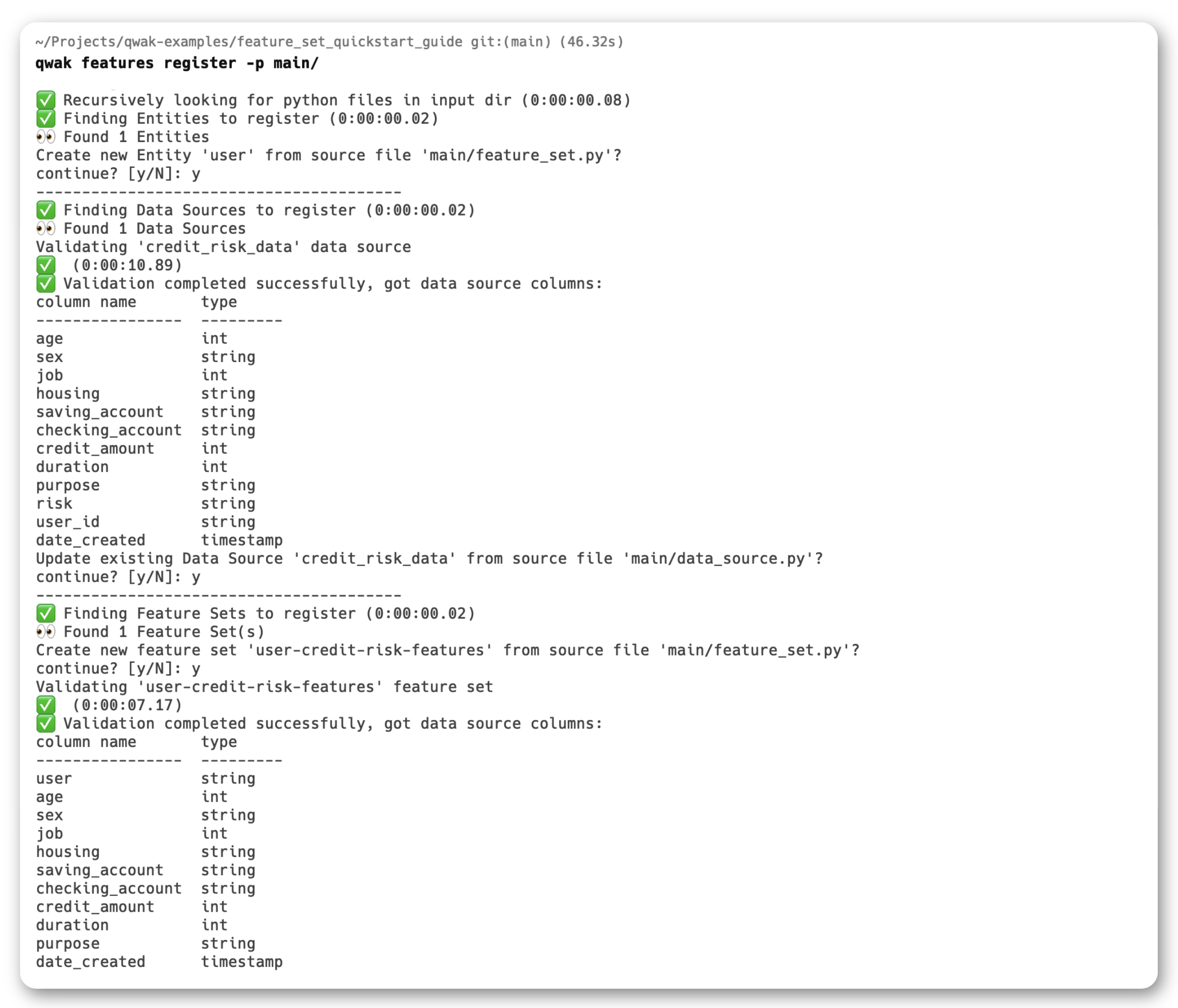
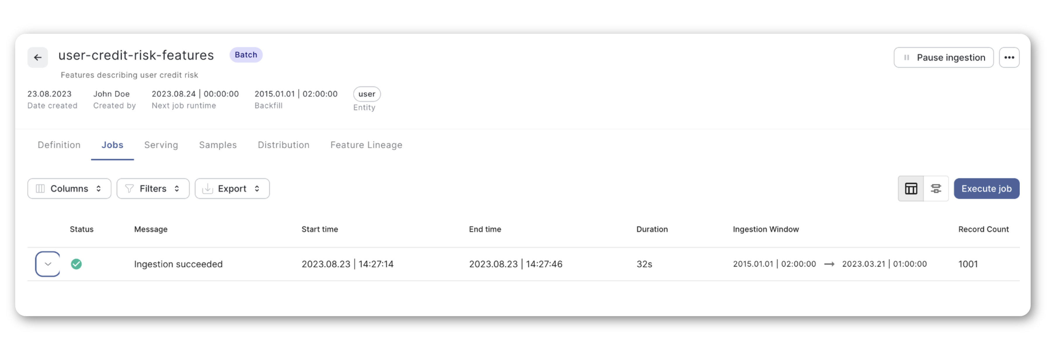
After successful registration, you should see your new Feature Set in the JFrog ML UI.
You can also manage the Feature Set in the JFrog ML UI, checking the status of processing jobs, querying the data, and exploring feature distributions.
Consume Features for Batch Model Training
After successful Feature Set registration, consuming its features for batch processing is straightforward.
Let's consider a generic FrogMlModel that requires data from the new Credit Risk Feature Set for model training and validation purposes. To achieve this, use the JFrog ML OfflineClientV2's get_feature_range_values() method as in the following example.
-
Initialization: Initializes an instance of the OfflineClientV2 class.
from frogml.feature_store.offline import OfflineClientV2 offline_client = OfflineClientV2() -
Features: Defines a list of features to retrieve from a specific feature-set.
from frogml.core.feature_store.offline.feature_set_features import FeatureSetFeatures features = FeatureSetFeatures( feature_set_name='user-credit-risk-features', feature_names=['checking_account', 'age', 'job', 'saving_account', 'sex'] ) -
Date Range: Specifies the start and end dates for which the feature values are to be fetched. In this example, the start date is set to January 1, 2021, and the end date is set to today's date.
from datetime import datetime feature_range_start = datetime(year=2021, month=1, day=1) feature_range_end = datetime.now() -
Fetch Features: Calls the
get_feature_range_valuesmethod on theoffline_clientinstance. The method returns the requested feature values for the specified key and date range, storing them in apandas.DataFrame.data = offline_client.get_feature_range_values( features=features, start_date=feature_range_start, end_date=feature_range_end )
The Offline Features are suited for model training and batch predictions and should be called in the build() method for training, or considering your model is deployed as batch, you can also call the client in the predict() method.
However, due to latency considerations, this is not a suitable solution for real-time predictions as we'll see in the next section.
# model.py
# Importing the FrogMlModel interface
from frogml import FrogMlModel

# Importing the Feature Store clients used to fetch results
from frogml.feature_store.offline import OfflineClientV2
from frogml.core.feature_store.offline.feature_set_features import FeatureSetFeatures

# Utility methods to log metrics and model parameters to FrogML Cloud
from frogml import log_param, log_metric
from datetime import datetime
import pandas as pd

# Constants
FEATURE_SET = "user-credit-risk-features"


# CreditRiskModel class definition, inheriting from FrogMlModel
class CreditRiskModel(FrogMlModel):

    # Class constructor - anything initialized here will be `pickled` with the Docker Image
    def __init__(self):
        < \..initialize - model.. >

        # Define the date range for data retrieval

    self.feature_range_start = date(2020, 1, 1)
    self.feature_range_end = date.today()

    < /..log - parameters.. >


# Method called by the FrogML Cloud to train and build the model
def build(self):
    # These are the specific features that the model will be trained on
    features = FeatureSetFeatures(
        feature_set_name=FEATURE_SET,
        feature_names=['checking_account', 'age', 'job', 'saving_account', 'sex']
    )

    # Lightweight client to access the OfflineStore
    offline_client = OfflineClientV2()

    # Fetch data from the offline client
    data = offline_client.get_feature_range_values(
        features=features,
        start_date=self.feature_range_start,
        end_date=self.feature_range_end
    )

    < \..train - and -validate - model.. >

< \..log - performance - metrics.. >


# Prediction method that takes a DataFrame with the User IDs as input, enriches it with Features and returns predictions
@frogml.api(feature_extraction=True)
def predict(self, df: pd.DataFrame, extracted_df: pd.DataFrame) -> pd.DataFrame:
    < \..prediction - logic.. >
To learn more about building and deploying models with JFrog ML, please check out our other QuickStart Guide.
Consuming Features for Real-Time Predictions
The JFrog ML OnlineClient provides a low-latency mechanism to query features in real-time without explicitly calling the client, unlike the OfflineClient.
To enable the OnlineStore to understand what features are required, define the ModelSchema object and the schema() function. In this case you can use the FeatureStoreInput to specify the feature set and feature names necessary for your prediction as in the example below.
# The FrogMlModel schema() function
def schema(self) -> ModelSchema:
  model_schema = ModelSchema(inputs=[
        FeatureStoreInput(name=f'{FEATURE_SET}.feature_a'),
        FeatureStoreInput(name=f'{FEATURE_SET}.feature_b'),
        FeatureStoreInput(name=f'{FEATURE_SET}.feature_c')
        ])
  return model_schema
When calling the predict() method, you only need to pass the query DataFrame (df), the rest of the features necessary for prediction are pulled by the feature_extraction functionality from the JFrog ML api() decorator which queries the OnlineStore automatically.
This way, df will be populated by the external service calling the predict() endpoint, and extracted will be enriched with the necessary features according to the model schema defined earlier.
# The FrogMlModel api() decorator with feature extraction enabled
@frogml.api(feature_extraction=True)
def predict(self, df: pd.DataFrame, extracted_df: pd.DataFrame) -> pd.DataFrame:

  # Call the prediction on the OnlineStore extracted_df DataFrame
  prediction = self.model.predict(extracted_df)

  return prediction
To put things in context, here's a generic FrogMlModel class using the Online Feature Store to enrich its predictions.
class CreditRiskModel(FrogMlModel):


# Class constructor - anything initialized here will be `pickled` with the Docker Image
def __init__(self):
    < /..init - model.. >


# Method called by the JFrogML Cloud to train and build the model
def build(self):
    < /..training - and -validation.. >


# Define the schema for the Model and Feature Store
# This tells JFrog ML how to deserialize the output of the Prediction method as well as what
# features to retrieve from the Online Feature Store for inference without explicitly specifying every time.
def schema(self) -> ModelSchema:
    model_schema = ModelSchema(inputs=[
        FeatureStoreInput(name=f'{FEATURE_SET}.checking_account'),
        FeatureStoreInput(name=f'{FEATURE_SET}.age'),
        FeatureStoreInput(name=f'{FEATURE_SET}.job'),
        FeatureStoreInput(name=f'{FEATURE_SET}.duration'),
        FeatureStoreInput(name=f'{FEATURE_SET}.credit_amount'),
        FeatureStoreInput(name=f'{FEATURE_SET}.housing'),
        FeatureStoreInput(name=f'{FEATURE_SET}.purpose'),
        FeatureStoreInput(name=f'{FEATURE_SET}.saving_account'),
        FeatureStoreInput(name=f'{FEATURE_SET}.sex'),
    ],
        outputs=[InferenceOutput(name=""score"", type = float)])
    return model_schema


# The FrogML API decorator wraps the predict function with additional functionality and wires additional dependencies.
# This allows external services to call this method for making predictions.

@frogml.api(feature_extraction=True)
def predict(self, df: pd.DataFrame, extracted_df: pd.DataFrame) -> pd.DataFrame:
    # Prediction method that takes a DataFrame with the User IDs as input, enriches it with Features and returns predictions

    # Cleaning the features to prepare them for inference
    X, y = utils.features_cleaning(extracted_df)

    print(""
    Retrieved
    the
    following
    features
    from the Online
    Feature
    Store:\n\n
    "", X)

    # Calling the model prediction function and converting the NdArray to a List to be serializable as JSON
    prediction = self.model.predict(X).tolist()

return predictionNote
For the full
FrogMlModelexample please consult the Github Gist Repository.
Testing your Model
JFrog ML offers you multiple options to test your models, locally, where you can benefit from a fast feedback loop, as well as query live model results to test your model in a production setup.
Local Testing
Please use the test_model_locally.py file to run the model locally on your laptop using the JFrog ML run_local functionality.
python test_model_locally.pyLive Model Testing
Once you have a working version of your model, please run the test_live_model.py file to use the JFrog ML RealTimeClient and query your live model endpoint.
python test_live_mode.py <your-model-id>Troubleshooting
This section could address common issues that you might encounter and how to resolve them. For example:
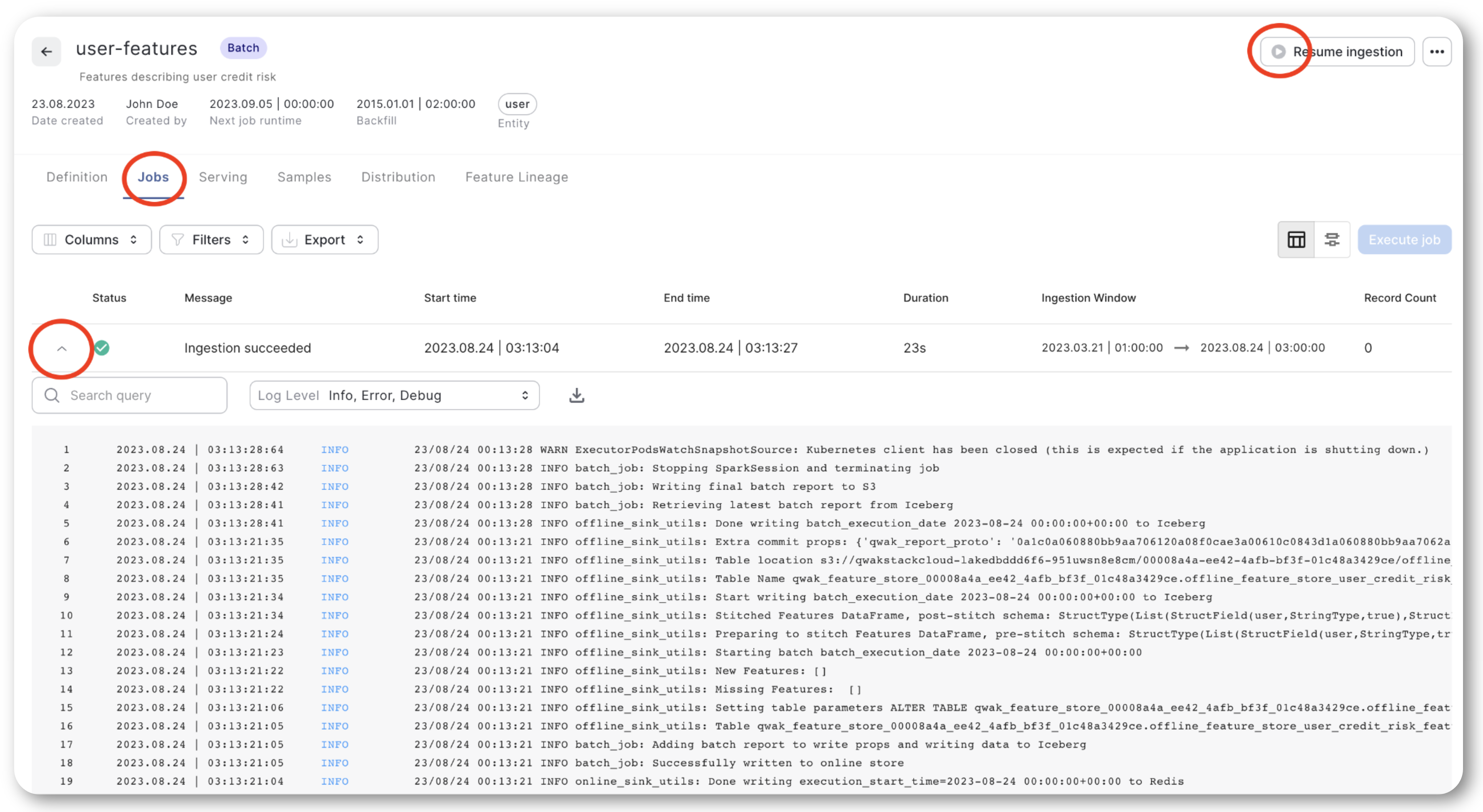
FeatureSet Pipeline Fails
If your data ingestion pipeline fails, the first step is to consult the logs for clues about the failure. Navigate to the 'Feature Set Jobs' section in the JFrog ML Dashboard, as shown below.
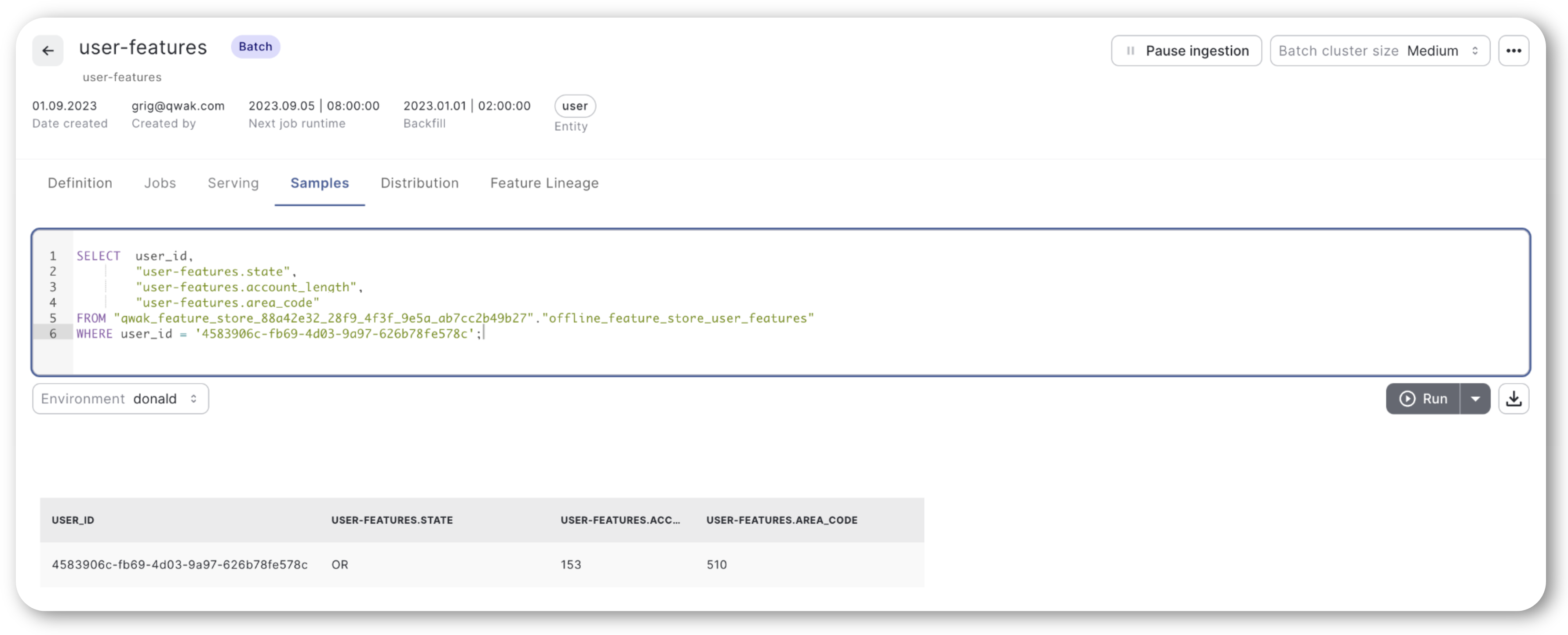
FeatureSet Querying
If you find that the Offline or Online client isn't retrieving any rows for a given key, you can verify the data exists in the JFrog ML UI under the 'FeatureSet Samples' section using an SQL query.
Note: When constructing your query, make sure to enclose column names in double quotes and prefix them with feature-store.feature, as shown in the example below.
Conclusion
In this comprehensive guide, we've walked you through the process of integrating JFrog ML Feature Store with Snowflake to manage and serve machine learning features effectively. From setting up prerequisites to defining the feature sets, we've covered all the essential steps. We also delved into the specifics of consuming features for both batch and real-time machine learning models.